Image Classification for Fashion MNIST
- Hindavi Churi
- Nov 7, 2022
- 9 min read

About
In this project, we will look how supervised learning algorithms help us to classify personal fashion apparel images after training data from the Fashion mnist dataset. Various Supervised learning models are trained, tuned, and tested to see the correctness it shows towards classifying. Depending on the aim, we compare various models and select the one that proves to satisfy the needs. In the end, the best suitable model is tested with real life fashion apparels to conclude how correct our model can classify.
Data
The Fashion MNIST data contains 60,000 images of fashion apparel for training and 10,000 images for testing which are loaded from keras datasets using TensorFlow framework. All the images are grayscale images and has a dimension of 28*28. Below picture depicts how these images look like,

As you can see, there are 10 different types of fashion apparel and our task is to classify the image into one of these labels.
Data pre-processing
The initial dataset consists of images which has a dimension of 28*28. However, we cannot use such 2D images for training and that brings us to pre-process the data before feeding it to the model for training. The data is already in the form of array, meaning, the pixel values from the images are already translated into an array with the help of NumPy library. These data are further flatten out to transform the 2D image array to 1D array. As the images are grayscale, the values of each pixel value lies in the range of (0,255). There is no issues with going ahead with these processed data, however to accelerate the computation of the model training, we will normalize the data using the Mean-Max scaling. The result of such transformation will give us values lying in the range of (0,1). We do the same transformations for both training and testing data.
Hyperparameter tuning
Hyperparameter tuning is one of the important part of any model training. It helps us find important hyperparameters which upon using with that model ensures best possible outcome for that data. Each model has different set of hyperparameters and hence we need to perform tuning each time for each model training. For this project, we have used Randomized Search method. The purpose of using this method is the data size of the training set. As the training set is large, tuning parameters for each possible value from the list of parameters may take huge amount of time calculated in days. Hence, to get faster results we use Randomized Search method picks values from the defined parameters randomly for tuning, thereby reducing more than half of the time for training.
Cross-validation
Cross-validation is an important aspect in order to discover whether our model is overfitting or not. Overfitting can be worrisome as the model may show best results for training data but will tremble down on testing data. Overfitting is caused when the model is trying to train complex data and wants to capture every aspect of the data as it is, and blanks out when new, real-life data is presented. Hence, in order to avoid overfitting or underfitting in that sense, where the model is not able to learn much; we perform cross-validation on the data. It is a process where the training data is divided into parts and uses some of its part for training and rest of the part for testing a couple of times. We use Stratified Cross-Validation on the training data. Stratified method divides data into k parts and uses k-1 combined parts for training and the left-out part for testing for k times. The advantage of using this method over others is that the divided parts contain equal ratio of classified data. This ensures impartial training of the data. For this project we divided our data into 3 parts, 2 parts for training and left out part for testing.
Evaluation Metric
Accuracy is the metric that is given first priority for this project. Since the project contains balanced data ,ie, each class has equally no of images to train and test on, accuracy will our ultimate deciding factor for the best model. Another reason is that the aim of the project is to identify the images correctly into classes and we are concern about the number of the correct predictions. The next priority is given to precision and recall to measure the correctness on how many classes that are predicted are actually right and how much it quantifies. Using such metrics is crucial for understanding how the images can be predicted into certain groups and its distributions.
Classification Models and their performance
Logistic Regression
Logistic Regression model gives out the probability of images for each class and the final output is classified as the one with the highest probability value. Initially we train and test the model with default hyperparameters and the accuracy comes out to be 84.45%. The hyperparameter tuning used for this model are penalty, type of solver and C value. We tune the model for 10 iterations. The best set of hyperparameters and the best accuracy score is shown below,
Best parameters for Logistic Rgeression: {'solver': 'lbfgs', 'penalty' : 'l2', 'C': 0.1}
Best Cross-validation score for Logistic Regression: 0.8563666666666667
We use best parameters for model and predict the test data. The accuracy of the model comes out to be 84.61%.
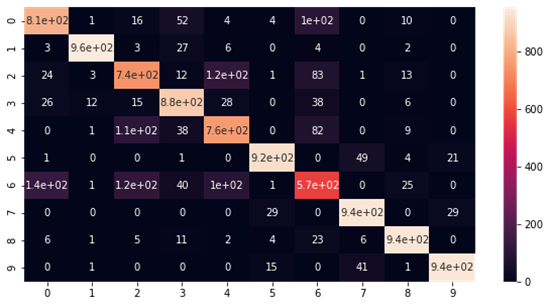
We can see from the confusion matrix that minimum no of correct predictions is for class 6, Shirt, and considerable amount of images are predicted as class 0(Top/T-shirt), class 2(Pullover) and class 4(Coat).
Multinomial Naïve Bayes
The Multinomial Naïve Bayes model gives out the likelihood of each class for the given image and outputs the class with the greatest chance to be correct. The initial evaluation score for default hyperparameters is 65.52%. The hyperparameter used for tuning is just the Alpha value. The best value for alpha and the best accuracy score is shown below,
Best parameters for Multinomial Naive Bayes:  {'alpha': 0.01}
Best Cross-validation score for Multinomial Naive Bayes:  0.66685
We use the best value for the model and predict the test data. The accuracy of the model comes out to be 65.53%. The difference between the initial naïve model and tuned model is negligible and almost same.

From the confusion matrix, we can depict that predictions for class 5(Sandals) and class 6(Shirt) are worst with more prediction count lying in the other class. Also, the prediction for class 6 seems to be confused into many other classes and shares that the model just can’t seem to predict shirt clearly most of the time and is confused.
K-Nearest Neighbours model
The K-Nearest Neighbours model gives the output based on the majority of the classes lying near the test sample among the K neighbours. For the initial evaluation, we check score for different k alternate neighbours between 7 to 31 and rest with the default hyperparameters. The best evaluation score among the k values is 84.95% for k=11. The hyperparameters for tuning are n neighbours and metric used for calculating the similarity. The best hyperparameter values and their accuracy score is shown below,
Best parameters for K-Nearest Neighbors Classifier:  {'n_neighbors': 11, 'metric': 'euclidean'}
Best Cross-validation score for K-Nearest Neighbors Classifier:  0.8465666666666666
The prediction score on test data using the best possible model is 84.95% which is same as initial model with default set of hyperparameters. Hence, we see no change in the model and flag the default model for KNN as best model for KNN.

From the confusion matrix, we can see that the class with maximum variations in prediction is class 6(Shirt). Class 4(Coat) and class 5(Sandal) has a little variation which is considerable.
Support Vector Machine model
The SVM model maps the data to high dimension space in order to categorize it as separable as possible and classifies the sample point into one of the classes based on its location in the space. The initial model with default hyperparameter gives evaluation score of 88.28%. The hyperparameters used for this model are C value, gamma value and type of kernel. The best hyperparameter values and their accuracy score are shown below,
Best parameters for SVM Classifier:  {'kernel': 'poly', 'gamma': 0.1, 'C': 0.1}
Best Cross-validation score for SVM Classifier:  0.8789000000000001
The prediction score for the test data using the best tuned model is 88.07%. Here, even though the default model gives slightly better result, it may be result of overfitting.

For SVM we can see that most of the classes are predicted correctly with high true positive values. However, class 6(Shirt) predictions are comparatively weak and shows a little diversion and mixes it up with class 0(Top/T-shirt). Also, class 4(Coat) shows few diversions with class 2(Pullover).
Decision Tree model
The Decision tree model gives out the output which follows it from the top of the branch until its last leaf where the classification is decided. The default model score for decision tree is 78.91%. The hyperparameters used for tuning are max depth up to which the tree should expand, the max features to be considered, the min sample leaf and min sample split. The best tuned model score along with the best set of values for the hyperparameters is shown below,
Best parameters for Decision Tree Classifier:  {'min_samples_split': 8, 'min_samples_leaf': 2, 'max_features': 'auto', 'max_depth': 120}
Best Cross-validation score for Decision Tree Classifier:  0.7791499999999999
The prediction score for the test data using the best tuned model is 78.22%.

For Decision Tree, many classes are showing poor to fair correct predictions. The worst of all is predictions for class 6(Shirt) with only half True predictions. It apparently is misclassified into class 0(Top/T-shirt), class 2(Pullover) and class 4(Coat). Class 4(Coat) and Class 2(Pullover) also has poor prediction score with some diversions.
Random Forest model
The Random Forest model as the name suggest is a forest of randomly produced decision trees form the data and the output for classification is taken as the majority count. The initial default hyperparameter model gives out the evaluation score of 87.64%. The hyperparameters used of tuning are n estimators for defining no of decision trees to be produced, and the rest are same as that of decision tree. The best tuned model score along with the best set of values for the hyperparameters is shown below,
Best parameters for Random Forest Classifier:  {'n_estimators': 400, 'min_samples_split': 2, 'min_samples_leaf': 1, 'max_features': 'auto', 'max_depth': 100}
Best Cross-validation score for Random Forest Classifier:  0.88205
The prediction score for the test data using the tuned model is 87.81% which is slightly better than default model.

For Random Forest Classifier, Class 6(Shirt) is again has poor prediction score with many diversion into class 0 and class 2. All other classes have a decent prediction score.
MLP model
The Multilayer perceptron model is a kind of neural network model which focuses on creating no of neurons and layers and training its data and finally giving out the result using some deciding activation function. The initial default hyperparameter model gives out the score of 88.24%. The hyperparameters used for tuning are hidden layer sizes, activation function, type of solver, alpha value, and the learning rate. The best tuned model and its best score are shown below,
Best parameters for MLP Classifier:  {'solver': 'sgd', 'learning_rate': 'constant', 'hidden_layer_sizes': (20,), 'alpha': 0.001, 'activation': 'tanh'}
Best Cross-validation score for MLP Classifier:  0.8685499999999999
The prediction score for the test data using the tuned model is 86.61%.

With the trend, Class 6(Shirt) has diversions which are classified into other classes majorly into class 0(Top/T-shirt) and class 2(Pullover). Class 2(Pullover) and class 4(Coat) show that they are sometimes classified into each other.
Model comparison
We compare all the model side by side to see how can we decide the best model. Shown below is a graph to help compare the model side by side,

The above graphs, compares the precision and recall scores for all the models. All the models have poor precision recall score for class 6. However, SVM and Random Forest has comparatively fair precision/ recall scores for class 6 and excellent scores for other classes. Hence, we mark these two models as potential candidates for best model for further testing.
Now, we look towards the accuracy to be our ultimate factor in deciding the best model. Refer the below graph for better understanding,

We compare the accuracy scores for all the models. Each model has two accuracy scores, Initial default score and final tuned score. As SVM and Random Forest being our potential candidate for being best, we can clearly see that SVM beats Random Forest slightly to become best model giving an accuracy of 88.07%. Hence, we select SVM as our best model and proceed further for testing real-life images.
Real life images processing
We used 10 different images based on each class as our real-life testing data. The images are of equal dimensions in square format and with applied background for better understanding. The images are sampled down to 28*28 dimension and further converted to a grayscale image. The images after processing looks like this,

The images are further flattened out and normalized same as before for testing with our best model.
Results
Using our best classification model, SVM, for given 10 test images, we were able to classify 7/10 images correctly.

The ones that are not identified are sneakers, ankle boots and pullover. Both Sneaker and ankle boot are predicted bag which can indicate that the images taken lacks contrast and details and the model depicts it as almost a square and predicts bag for them. Also, the pullover is predicted as shirt and one of the reasons can be contrast and clarity.
Source Code
Conclusion
Fashion MNIST images were processed, trained and tested using various classification models. The classification models were trained well such that no overfitting done and tuned to it ultimate hyperparameters. The best model was selected looking at various evaluation metrics such as precision, recall and accuracy being the ultimate deciding factor. SVM outperforms all other models after scrutiny and was further used for testing real-life images. All 10 unique class images from real-life were tested using SVM with 7 being detected correctly.


Comments